Square Potential Well

July 15, 2026

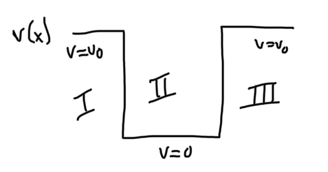
One of the most basic quantum mechanics problems is the square potential well. The basic description is that there is a quantum particle in a small well made of a potential field. The particle only has one degree of freedom, so this is considered a one-dimensional problem. First, we start with a drawing to visualize the problem.

Problem Definition

We have three regions, I, II, and III. Our goal is to find the wavefunction of our particle in each of the regions. In regions I and III, the potential is $V_0$ , and in region II, the potential is 0. Mathematically, we define this:

\begin{align}V(x)&amp;=0, &amp;|x|\le a\\ &amp;= V_0,&amp;|x|\ge a \end{align}

We are going to be working in the $X$ basis, and the goal is to find the allowed energy states.

Solving the Problem

We are going to start with the Schrödinger equation:

-\frac{\hbar^2}{2m}\frac{d^2\psi}{dx^2}+V(x)\psi=E\psi

rearranging this, (as well as writing the second spatial derivative of the wavefunction as $\psi”$ ), we get

\psi”-\frac{-2m(V-E)\psi}{\hbar^2}=0

This is a differential equation that will be the starting point for each section. This is a type of differential equation that will always result in an exponential. We will begin with section III.

We now have the equation

\psi_{III}”-\frac{-2m(V_0-E)\psi_{III}}{\hbar^2}=0

Solving, we get

\psi_{III}=Ae^{-\kappa x}+Be^{\kappa x}

where

\kappa=\sqrt{\frac{2m(V_0-E)}{\hbar^2}}

We can similarly solve sections I and II to get the equations

\begin{align} \psi_I=Ge^{-\kappa x}+De^{\kappa x}\\ \psi_{II}=Ee^{ikx}+Fe^{-ikx} \end{align}

where

k=\sqrt{\frac{2mE}{\hbar^2}}

We have some boundary conditions on any wave function. A wave function must be normalizable, meaning that it must be square integrable, so it has to go to 0 on both ends. Therefore, in sections I and III, we can impose the restrictions $\lim_{x\to\pm\infty}\psi_{I,III}=0$ . This gives us $B=G=0$ . With this information, we can change the equation for region II to

\psi_{II}=E\sin{kx}+F\cos{kx}

We also need the wavefunction to be continuous, so we can equate the functions for regions I and II at $x=-a$ and the functions for regions II and III at $x = a$ . We also have to equate their derivatives at the same points. Doing this, we get two types of equations, called symmetric and antisymmetric. The symmetric case is where $A=0$ and $G=H$ and the antisymmetric case is where $B=0$ and $G=-H$ . For the symmetric case, we get

\kappa=k\tan(ka)

and for the antisymmetric case we get

\kappa=-k\cot(ka)

Since both $k$ and $\kappa$ depend on energy, this means that there cannot be arbitrary energy levels in this situation. This is where the “quantum” part of quantum mechanics comes from; energy is not a continuous spectrum, but quantized into discrete levels.

Going back to the initial values of $k$ and $\kappa$ , we can see that, as $V_0\to\infty$ , $\kappa\to\infty$ . Therefore, we must find the values of $k$ where $1/\kappa\to0$ .

\begin{align} -\frac{1}{k\cot ka}&amp;=0\to ak=n\pi\to k=\frac{n\pi}{a}\\ \frac{1}{k\tan ka}&amp;=0\to k=\frac{\pi}{a}\left(n+\frac{1}{2}\right) \end{align}

The best way to solve from here is to graph them. First, we note that

k^2+\kappa^2=\frac{2mV_0}{\hbar^2}

This will graph a circle for us, based on the value we have for $V_0$ . Now, we choose our coordinate system. We choose $\alpha=ka$ , $\beta=\kappa a$ . We now have the equations

\begin{align} \beta=\alpha\tan\alpha\\ \beta=-\alpha\cot\alpha\\ \alpha^2+\beta^2=2\pi^2 \end{align}

We plot these as orange, blue, and green, respectively.

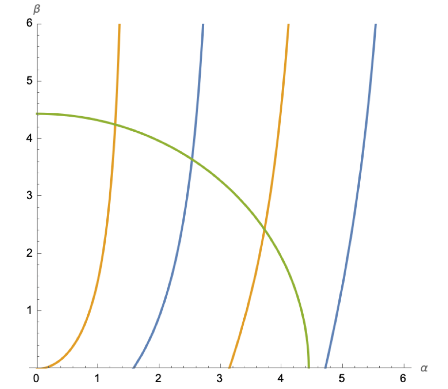
For this arbitrarily chosen value of $V_0$ (which, in this case, happens to be $\frac{\hbar^2\pi^2}{ma^2}$ ), we have three instances where the graphs cross the circle. These are called “bound states,” which refers to any states where the energy leaves the particle inside of the well. “Unbound states” are what we call the states where the energy level allows the particle to be above the well.

At this point, all we have to do is solve the graph, which can be done in a few ways. Any way that gives you the intersection of the two lines will do. Commonly, you’ll want to use a numerical method and a computer to do this, as it may be hard or impossible to do analytically.

What’s Next?

After doing this problem, there are a few different things you can try. There is the particle in a box, which is the same problem, but with $V_0=\infty$ . The particle in a box tends to be easier, but I personally find the potential well to be more informative. You can also try to solve the problem when the left and right side potentials are different. Another interesting thing you can try is to increase the number of dimensions; instead of just the x direction, try x and y. Eventually, you can build up to finding the energy states of a hydrogen atom, which adds a lot of complexity, but is not out of reach for people who understand the concepts and math of this problem.